Hiding in plain sight …

My final post of 2023 (“Call me by my name …”) looked at the fraught business of putting names onto microscopic organisms, dividing the problem into limitations of knowledge and practical challenges.  Limitations of knowledge mean that there is no single definitive work to which we can refer.  Practical challenges include limitations of our equipment but also our capacity to access an increasingly diffuse literature, some of which sits behind internet paywalls.  At the intersection of these two challenges sit “cryptic species”: those that we know exist, but which cannot reasonably be differentiated with light microscopy.   

In many parts of the world, diatoms are used as part of statutory assessments of freshwater health so it is worth asking ourselves just how much extra sensitivity we may unlock by accessing all this unknown and hidden information about diatom species.  How might we do that?   The dominant approach to naming diatoms uses characteristic shapes and structures to differentiate species so we need to find a way of differentiating all the variety within diatoms that does not rely upon our ability to see and describe this variation.  The answer lies in molecular genetics where, rather than using morphology, we differentiate using sequences of DNA.  Until now, though, people have mostly tried to link these sequences to traditional names defined by (you’ve guessed it …) our inherently-flawed system of shape- and character-based taxonomy.  Suppose that, instead of this, we did all steps required of DNA-based identification except for that final one where we fitted the outputs to traditional names.  How would that change the situation?

About 2800 diatoms have been recorded from the UK and Ireland, based on traditional shape-based species concepts.  Our study, based on a dataset of 1220 samples from rivers all around the UK, we found 4036 distinct entities.  Not all of these will be “species” in the traditional sense but, on the other hand, some of the sequences we identified may encompass more than one species.  Metabarcoding uses relatively short fragments of DNA from a single gene whereas taxonomists would work with longer lengths of two or more genes as well as morphology.  However, this does at least offer us a ballpark figure for how many diatom species we are yet to find.  Very roughly, for every two diatom species we already know about, there is one more waiting to be described.  As our dataset comes from rivers, we are probably missing some of the diversity in lakes and soil, so the true figure may be even higher. 

Our primary purpose in doing these analyses was to see if we could improve the models we use for statutory assessments.   Way back in 1995 when I put together the first version of the Trophic Diatom Index (TDI), it explained 63 percent of the variation in the river phosphorus gradient.  Since then, the TDI has gone through several iterations as species have been added and coefficients have been tweaked but, until this study, we always used traditional diatom species names (even when using molecular genetics to generate our data). Now, almost 30 years since the first version of the TDI, we generated a model that bypassed traditional names (and all the limitations this introduces) and produced a model which explained 72 percent of the variation in the nutrient gradient.   

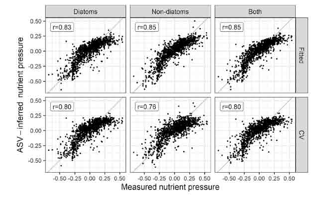
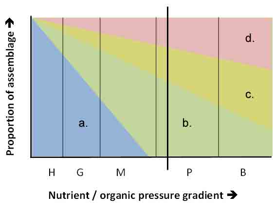
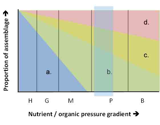
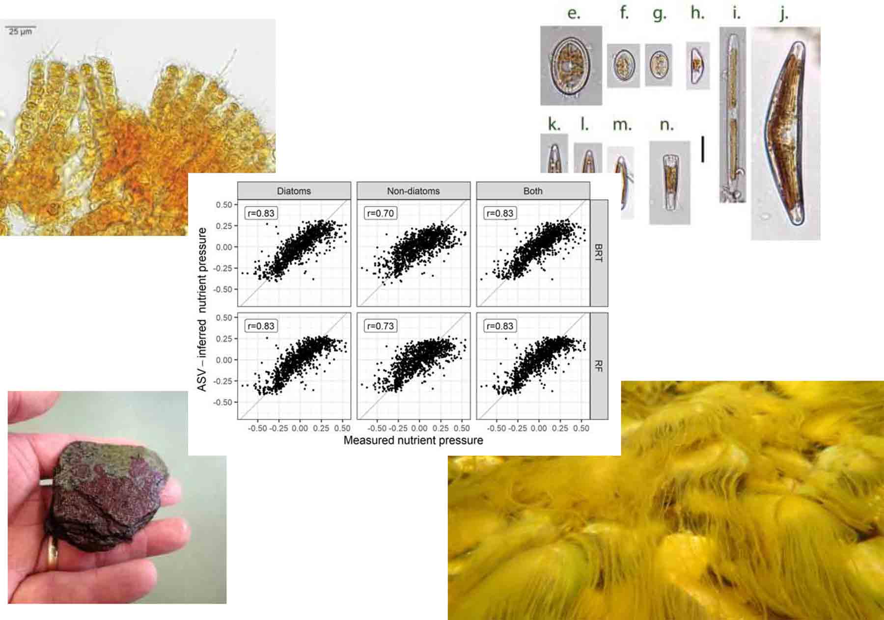
Results of weighted-average (WA) predictive models, showing relationship between observed and ASV-inferred nutrient pressure for diatoms and non-diatoms, and both (combined) (left). Upper plots show relationship for model fits, lower plots show results after 2-fold leave-out cross validation.  See Kelly et al. (2024) for more details.  The figure at the top is the graphical abstract from this paper.

This is not a perfect statistical comparison, but it reflects the reality of the situation.  We captured most of the diatom v nutrient signal with our relatively crude approach back in the early 1990s and have spent the last 30 years crawling slowly towards the asymptote.  We calculated that the strongest model we could compute with the (imperfect) chemical data we are given is, in theory, 86 per cent.  However, that assumes no other factors are influencing the diatoms and we know that is not the case.  Whilst strong models should allow regulators to better predict the ecological benefits of reducing phosphorus, there is also a danger that we become blind to the complexity of river systems in the process of developing these.  

Our result suggests that, however hard taxonomists work to track down the 1200 or so “missing” species, this will add relatively little functionality to our current mode of assessment.  Of course, having a better idea of the diversity of the algae of Britain and Ireland is a worthwhile end in its own right, although some of this diversity will be “cryptic”, impossible to unlock with conventional microscopy.  The answer is to find new ways to use this rich source of information rather than refining existing approaches. 

The problem, as we attempt to unravel this diversity and explain it in terms that can be used when identifying diatoms using a microscope is that we are encountering many of these 1200 “missing” species all the time.  They are hiding in plain sight, but we are not recognising them as discrete species because no-one has told us how to differentiate them from their near-neighbours.  The challenge for taxonomists is to capture the characteristics of these unambiguously using words and pictures, when many of the characters visible with the light microscope will overlap with those of near neighbours.  Otherwise, the sensitivity gained by extra knowledge will be cancelled out by error introduced by mis-identifications resulting from ambiguous and diffuse literature.  We are almost back where we started, still channelling the spirit of van Leuwenhoek four hundred years ago, struggling to make sense of realms that sit at the borders of our awareness … 

References

Kelly, M. G., & Whitton, B. A. (1995). The trophic diatom index: a new index for monitoring eutrophication in rivers. Journal of applied phycology 7: 433-444.

Kelly, M. G., Mann, D. G., Taylor, J. D., Juggins, S., Walsh, K., Pitt, J. A., & Read, D. (2023). Maximising environmental pressure-response relationship signals from diatom-based metabarcoding in rivers. Science of The Total Environment 914: 169445.

Some other highlights from this week:

Wrote this whilst listening to:  music referred to in Do Not Say We Have Nothing (see below).  In particular, Pink Floyd’s Set the Controls to the Heart of the Sun and Mahler’s Das Liede von der Erde, both of which have words derived from ancient Chinese poetry.  

Currently reading:  Do Not Say We Have Nothing by Madeleine Thien, a novel that spans Chinese history from the Sino-Japanese war to Tiananmen Square in 1989.  

Cultural highlight:  Mercury-prize nominated Irish band Lankum at the Boiler Shop in Newcastle.  Traditional folk instrumentation but with enough of a nod to My Bloody Valentine to make me want to gaze at my shoes at times.

Culinary highlight: fillets of sea bass roasted and served over a bed of pan-fried fennel. A recipe from a book of Venetian recipes that we had forgotten we had.

All change …

For the first time since the start of the pandemic I’m travelling to a conference, to give a plenary talk about the UK’s experience with applying metabarcoding to ecological assessment.   I’ve not written about this on the blog for some time (see “Dispatches from Plato’s cave …”) so I’m taking the opportunity of preparing a talk, and sitting around in transit lounges, to summarise some of my thoughts.  I’ve also put in a few of my photos from this trip to break up the text.

The UK was the first country in Europe where the regulatory bodies got involved, alongside academics, in the application of metabarcoding to environmental regulation.  From the outset, we have had funding from the government agencies responsible for regulation, and had their representatives looking over our shoulders as results started to emerge.  That was mostly a constructive relationship between research scientists, but we had more than our fair share of tense moments, sometimes feeling like pawns in wider inter- and intra-agency squabbles.  What I came to realise, however, was that these discussions about the science often missed broader issues about how the new technology would affect whole organisations.  The introduction of metabarcoding, I came to see, was a case study in managing change in organisations that make decisions using ecological data.  

I wrote about this in an online paper a few years ago, and some of my reflections gained further traction when I listened to an episode of Tim Harford’s excellent Cautionary Tales podcast [https://timharford.com/2019/12/cautionary-tales-ep-6-how-britain-invented-then-ignored-blitzkrieg/].  This is about tank warfare rather than ecology, explaining how, he following the invention of the tank, commanders in the British army tried to fit it into the existing approaches to warfare rather than redesigning battle formations to make full use of the tank’s capabilities.   It was left to the German army to do this more radical restructuring in the 1930s, resulting in the “Blitzkrieg” tactics that overrun much of Europe in matter of weeks in 1940.  Harford related these changes back to a paper on business strategies for managing change.   This classified change in two ways: whether or not the core concepts and components that underlay processes in an organisation were changed by a new innovation, and whether or not this affected the linkages between these, which can be visualised as a table:   

Over the course of this podcast, I realised that the same analysis could be applied to the work that we were doing.  Until our metabarcoding projects, the Environment Agency had been using light microscopy to analyse diatoms for about 20 years, using an index that I developed in the early 1990s.   That first version had undergone several changes over the years as our understanding techniques and taxonomy has developed, but these could all be regarded as “incremental innovation” insofar as each development reinforced the way that the data produced was used by the organisation as a whole.   Environment Agency managers, meanwhile, were tinkering with linkages, moving from a structure where almost every area had in-house capability combined with local knowledge to one where diatom analyses were focussed around a few “hubs”.  That counts as an “architectural innovation” because the pathway from sample collection to the use of the data in decision-making changed.  

Arch of the Sergii, a Roman triumphal arch in Pula, dating from approximately 27 BC.  The photograph at the top of the post shows the first century Roman Arena.

When we started the metabarcoding project, there was an assumption that, at some point, metabarcoding would replace analysis by light microscopy, much as you might upgrade a component in your computer: the old component is taken out, the new one dropped in, and everything proceeds as before. In Henderson and Clark’s terminology, this was a “modular innovation”.   Unfortunately, this turned out to be a naïve assumption. Replacing light microscopy by metabarcoding has implications that go beyond the analysis of samples and is, in fact, another example of “architectural innovation”.  The “linkages” (how data/information flowed through the organisation) also need to change if full value from the new method is to be obtained. Here are three examples:

• Area staff found they had much less agency in the production of data in the metabarcoding era.   There were often long lags between samples being collected and results being available because samples were batched up and sent to remote laboratories where finite analytical capacity created a bottleneck at the times of year when samples were collected.   Previously, area staff could either prioritise particular samples themselves (if they were investigating a local river, for example) or telephone the people that were doing the analysis and ash them to fast-track these samples. 
  
• Time spent collecting and analysing samples is valuable unstructured learning that gives ecologists the experience that they need to interpret data.   You slowly learn to associate particular organisms with certain habitats and, gradually, build up a “sixth sense” about when you have encountered an unusual sample.  This was particularly the case in the UK system where a biologist might have had quite detailed knowledge (invertebrates, macrophytes, diatoms) of a single catchment.   In the metabarcoding era, the first time a biologist encounters an organism is as an entry in a spreadsheet or database containing processed sequencing output.   One option is to automate data interpretation; however, this raises more questions.  What is gained and, more importantly, what is lost by not having expert field ecologists involved at this stage?
  
• Finally, metabarcoding for ecological assessment is still a very young science and new developments appear regularly in the literature.  However, you cannot keep tinkering with a system that, ultimately, drives multi-million pound/dollar/euro investment decisions.  The regulators want to “lock down” a particular method in the interests of stability and transparency.  However, in the time it takes to pass all the stages of approval in government bureaucracy, improvements on the method are likely to have become available.  Given that we know that there is always uncertainty in predictions of ecological status, any improvement ought to bring us, incrementally, towards more robust decisions.  Too much faith in “stability” simply entrenches avoidable errors.   There is, in the UK, recognition of a need to embrace “incremental innovation” within regulation, but the process is not very systematic and certainly not regular enough.   At the moment, the mantra of “stability” is putting the cart before the horse, and some genuinely bad decisions will slip through the net as a result.   

I tried to capture some of these issues in the title of my paper.  Characterising molecular ecology as “fast-moving” is not controversial.   Characterising environmental regulation as “slow-moving” might appear pejorative but there are good reasons why this should be the case.  None of us would be happy if the speed limits changed overnight on our local roads without good reason and due warning and the same applies to environmental regulation.   This mismatch between science and regulation, however, means that the gap between what is possible and what is allowed is set to widen.  Up to now, we have been expected to squeeze the science into outdated regulatory models.  What we need to think about now is how regulation can evolve to embrace this new potential.

References

Henderson, R.M. & Clark, K.B. (1990).  Architectural innovation: the reconfiguration of existing product technologies and the failure of existing firms.  Administrative Science Quarterly 35: 9-30.

Kelly, M. (2019). Adapting the (fast-moving) world of molecular ecology to the (slow-moving) world of environmental regulation: lessons from the UK diatom metabarcoding exercise. Metabarcoding and Metagenomics, 3, e39041. [https://mbmg.pensoft.net/article/39041/]

Santa Maria Formosa, a Byzantine chapel dating from the 6^th century.   The best views are from beside a busy road in bright sunlight.   The view from a nearby café was not as good but I was able to sit in the shade and sip beer whilst I sketched.

Some other highlights from this week: 

Wrote this whilst listening to: The Rest is Politics podcast with Alistair Campbell and Rory Stewart.  Strictly speaking, writing this blog was delayed while I absorbed unfolding political events in the UK.  The implications of economic and fiscal policy will have knock-on effects for all government departments and, therefore, for the subject I write about here.

Currently reading: Act of Oblivion, latest novel from Robert Harris book, set at the time of the Restoration and the revenge enacted on those responsible for the execution of Charles I.  

Cultural highlight:  See How They Run, whose plot involves murders on the set of Agatha Christie’s The Mousetrap.   Gentle, old-fashioned humour channelling the Ealing Comedies of yore.

Culinary highlight:  Currently in Croatia and eating hotel buffet food, which is plentiful though hardly a “highlight”. It has, however, removed any inclination to search out any IrIstrian cuisine that might otherwise replace this as the top gastronomic experience of my trip.

20:20 hindsight …

Last week saw the publication of a paper that has undergone a slow gestation through the year.   It’s an opinion piece published in the new open access journal Metabarcoding and Metagenomics and describes some of the lessons I learned during the development of a new diatom metric based on metabarcoding data.   The science behind these projects is written up in reports and papers, but that only tells part of the story.  Applied science needs a context, and my paper is more about how the new science fits into a wider process of managing change in large and ponderous government agencies.

That’s where my title comes from: “Adapting the (fast-moving) world of molecular ecology to the (slow-moving) world of environmental regulation”.   The new science of metabarcoding is developing fast and some of the assumptions that we made at the start of the project have now been overtaken by developments in methods.  Yet the regulatory systems into which these methods will be integrated need to be stable and continual “tweaks” to optimise the system would not be welcome.   “Ponderous”, in this context, is not necessarily a bad thing.  Imagine driving in your local area and finding all the speed limits had changed at the whim of an official and without any consultation or advance warning.  Finding a balance between these two needs: for the best possible methods and a stable basis for regulation seems to be one of the biggest challenges those of us with an interest in molecular ecology face over the next few years.

My own view, reflecting back over the discussions I’ve had over the past few years, is that this is possible, but that the UK’s environment agencies will need some major structural changes for this to come about.   As I was reviewing the proofs of the paper, I came across Tim Harford’s fascinating podcast Cautionary Tales and, in particular, an episode called “How Britain Invented, then Ignored, Blitzkrieg”.  The point he made in this episode was that improvements to individual components of a system (tanks, in his example) have little value if the overall architecture within which those components operate are not also regularly updated.   He cited a paper by Rebecca Henderson and Kim Clark which, had I seen it sooner, would have strengthened the principal argument in my paper.

Henderson and Clark’s examples were drawn from manufacturing industry, but we can use the same kind of language to make their framework relevant to ecological assessment.   Broadly speaking, an ecological assessment method (using diatoms, in this case, but it could also be invertebrates, macrophytes or fish) is one component in a larger decision-making “machine”.  Replacing the existing methods, based on specialist biologists painstakingly analysing samples to identify and enumerate the taxa present by one based on metabarcoding technology constitutes a “modular innovation”, using the terminology in the table below.   That might well work in some cases (replacing an analogue by a digital telephone, for example, doesn’t fundamentally affect the way we communicate with one another).  However, the question that Henderson and Clark were asking was what happens when an innovation interacts differently with other components, in which case a shift in the entire product design might be necessary.

A framework for defining innovation (after Henderson and Clark, 1990)

		Core concepts
		Reinforced	Overturned
Linkages between core concepts and components	Unchanged	Incremental innovation	Modular innovation
	Changed	Architectural innovation	Radical innovation

Harford used the comparative fortunes of IBM and Apple in his podcast (Henderson and Clark’s paper was written before the tech revolutions, otherwise I’m sure they would have done so too).  Apple did not invent the mouse or the graphical user interface, but they were able to fit these into a radical new architecture of components, opening up an enormous market for consumer-friendly gadgets.  IBM, by contrast, was the market leader for mainframe computers, but its thinking and organisational structures were so focussed on these that they were not nimble enough to adapt to this new world.

The question that arises when using metabarcoding in a regulatory capacity is whether this technology just constitutes a “modular innovation” or whether a broader refit of the organisations that use the technology is necessary in order to maximise their benefits. My argument is that metabarcoding constitutes a “radical innovation” partly because the way that individuals interpret  metabarcoding data is different to the way that they would traditional data, which means that the value that a biologist can add to evidence for a regulatory decision on his/her locale will change, and because the gathering of evidence by traditional means constituted an “unstructured training program” for freshwater biologists that gave them a broad awareness of freshwater ecology in their region.

Furthermore, the rate of development of these new technologies is such that a better way needs to be find of balancing innovation and regulatory stability beyond the very ponderous approach in force in the UK at the moment.  There are ways of doing this, but the mindset in the administrations needs to change before these can be implemented and there would also need to be more administrators to oversee this process, a big ask in a public sector still limping along on much reduced budgets.

One of the biggest lessons we learned was, in fact, that if you want to learn lessons you need to get stuck in and have a go.  There are plenty of review papers in the academic literature now saying how metabarcoding might be used for ecological assessment, and plenty of discussion about these new technologies within the hierarchies of the government agencies. But you can only go so far with theory: not all of the challenges we encountered were anticipated and, certainly, not all the assumptions that drove the original commissioning of the project turned out to be correct.   The only way of testing these was to take a step into the unknown.  We learned the hard way, but maybe future projects will benefit.

Reference

Henderson, R.M. & Clark, K.B. (1990).  Architectural innovation: the reconfiguration of existing product technologies and the failure of existing firms.  Administrative Science Quarterly 35: 9-30.

 

The Imitation Game

About a year ago, I made a dire prediction about the future of diatom taxonomy in the new molecular age (see “Murder on the barcode express …“).   A year on, I thought I would return to this topic from a different angle, using the “Turing Test” in Artificial Intelligence as a metaphor.   The Turing Test (or “Imitation Game”) was derived by Alan Turing in 1950 as a test of a machine’s ability to exhibit intelligent behaviour, indistinguishable from that of a human (encapsulated as “can machines do what we [as thinking entities] can do?”).

My primary focus over the past few years has not been the role of molecular biology in taxonomy, but rather the application of taxonomic information to decision-making by catchment managers.   So my own Imitation Game is not going to ask whether computers will ever identify microscopic algae as well as humans, but rather can they give the catchment manager the information they need to make a rational judgement about the condition of a river and the steps needed to improve or maintain that condition as well as a human biologist?

One of the points that I made in the earlier post is that current approaches based on light microscopy are already highly reductionist: a human analyst makes a list of species and their relative abundances which are processed using standardised metrics to assign a site to a status class. In theory, there is the potential for the human analysts to then add value to that assignment through their interpretations.  The extent to which that happens will vary from country to country but there two big limitations: first, our knowledge of the ecology of diatoms is meagre (see earlier post) and, in any case, diatoms represent only a small part of the total diversity of microscopic algae and protists present in any river.   That latter point, in particular, is spurring some of us to start exploring the potential of molecular methods to capture this lost information but, at the same time, we expect to encounter even larger gaps in existing taxonomic knowledge than is the case for diatoms.

One very relevant question is whether this will even be perceived as a problem by the high-ups.  There is a very steep fall-off in technical understanding as one moves up through the management tiers of environmental regulators.   That’s inevitable (see “The human ecosystem of environmental management…“) but a consequence is that their version of the Imitation Game will be played to different rules to that of the Environment Agency’s Poor Bloody Infantry whose game, in turn, will not be the same as that of academic taxonomists and ecologists.  So we’ll have to consider each of these versions separately.

Let’s start with the two extreme positions: the traditional biologist’s desire to retain a firm grip on Linnaean taxonomy versus the regulator’s desire for molecular methods to imitate (if not better) the condensed nuggets of information that are the stock-in-trade of ecological assessment.   If the former’s Imitation Game consists of using molecular methods to capture the diversity of microalgae at least as well as human specialists, then we run immediately into a new conundrum: humans are, actually, not very good at doing this, and molecular taxonomy is one of the reasons we know this to be true.  Paper after paper has shown us the limitations of taxonomic concepts developed during the era of morphology-based taxonomy.  In the case of diatoms we are now in the relatively healthy position of a synergy between molecular and morphological taxonomy but the outcomes usually indicate far more diversity than we are likely to be able to catalogue using formal Linnaean taxonomy to make this a plausible option in the short to medium-term.

If we play to a set of views that is interested primarily in the end-product, and is less interested in how this is achieved, then it is possible that taxonomy-free approaches such as those advocated by Jan Pawlowski and colleagues, would be as effective as methods that use traditional taxonomy.   As no particular expertise is required to collect a phytobenthos sample, and the molecular and computing skills required are generic rather than specific to microalgae, the entire process could by-pass anyone with specialist understanding altogether.  The big advantages are that it overcomes the limitations of a dependence on libraries of barcodes of known species and, as a result, that it does not need to be limited to particular algal groups.  It also has the greatest potential to be streamlined and, so, is likely to be the cheapest way to generate usable information.   However, two big assumptions are built into this version of the Imitation Game: first, there is absolutely no added value from knowing what species are present in a sample and, second, that it is, actually, legal. The second point relates to the requirement in the Water Framework Directive to assess “taxonomic composition” so we also need to ask whether a list of “operational taxonomic units” (OTUs) meets this requirement.

In between these two extremes, we have a range of options whereby there is some attempt to align molecular barcode data with taxonomy, but stopping short of trying to catalogue every species present.  Maybe the OTUs are aggregated to division, class, order or family rather than to genus or species?   That should be enough to give some insights into the structure of the microbial world (and be enough to stay legal!) and would also bring some advantages. Several of my posts from this summer have been about the strange behavior of rivers during a heatwave and, having commented on the prominence and diversity of green algae during this period, it would be foolish to ignore a method that would pick up fluctuations between algal groups better than our present methods.   On the other hand, I’m concerned that an approach that only requires a match to a high-level taxonomic group will enable bioinformaticians and statisticians to go fishing for correlations with environmental variables without needing a strong conceptual behind their explorations.

My final version of the Imitation Game is the one played by the biologists in the laboratories around the country who are simultaneously generating the data used for national assessments and providing guidance on specific problems in their own local areas.   Molecular techniques may be able to generate the data but can it explain the consequences?  Let’s assume that method in the near future aggregates algal barcodes into broad groups – greens, blue-greens, diatoms and so on, and that some metrics derived from these offer correlations with environmental pressures as strong or stronger than those that are currently obtained.   The green algae are instructive in this regard: they encompass an enormous range of diversity from microscopic single cells such as Chlamydomonas and Ankistrodesmus through colonial forms (Pediastrum) and filaments, up to large thalli such as Ulva.   Even amongst the filamentous forms, some are signs of a healthy river whilst others can be a nuisance, smothering the stream bed with knock-on consequences for other organisms.   A biologist, surely, wants to know whether the OTUs represent single cells or filaments, and that will require discrimination of orders at least but in some cases this level of taxonomic detail will not be enough.   The net alga, Hydrodictyon(discussed in my previous post) is in the same family as Pediastrumso we will need to be able to discriminate separate genera in this case to offer the same level of insight as a traditional biologist can provide.   We’ll also need to discriminate blue-green algae (Cyanobacteria) at least to order if we want to know whether we are dealing with forms that are capable of nitrogen fixation – a key attribute for anyone offering guidance on their management.

The primary practical role of Linnaean taxonomy, for an ecologist, is to organize data about the organisms present at a site and to create links to accumulated knowledge about the taxa present.    For many species of microscopic algae, as I stressed in “Murder on the barcode express …”, that accumulated knowledge does not amount to very much; but there are exceptions.  There are 8790 records on Google Scholar for Cladophora glomerata, for example, and 2160 for Hydrodictyon reticulatum.  That’s a lot of wisdom to ignore, especially for someone who has to answer the “so what” questions that follow any preliminary assessment of the taxa present at a site.  But, equally, there is a lot that we don’t know and molecular methods might well help us to understand this.   There will be both gains and losses as we move into this new era but, somehow, blithely casting aside hard-won knowledge seems to be a retrograde step.

Let’s end on a subversive note: I started out by asking whether “machines” (as a shorthand for molecular technology) can do the same as humans but the drive for efficiency over the last decade has seen a “production line” ethos creeping into ecological assessment.   In the UK this has been particularly noticeable since about 2010, when public sector finances were squeezed.   From that point on, the “value added” elements of informed biologists interpreting data from catchments they knew intimately started to be eroded away.   I’ve described three versions of the Imitation Game and suggested three different outcomes.  The reality is that the winners and losers will depend upon who makes the rules.  It brings me back to another point that I have made before (see “Ecology’s Brave New World …”): that problems will arise not because molecular technologies are being used in ecology, but due to how they are used.   It is, in the final analysis, a question about the structure and values of the organisations involved.

References

Apothéloz-Perret-Gentil, L., Cordonier, A., Straub, F., Iseili, J., Esling, P. & Pawlowksi, J. (2017).  Taxonomy-free molecular diatom index for high-throughput eDNA monitoring.   Molecular Ecology Resources17: 1231-1242.

Turing, A. (1950).  Computing machinery and intelligence.  Mind59: 433-460.

The multiple dimensions of submerged biofilms …

My recent dabbling and speculation in the world of molecular biology and biochemistry (see “Concentrating on carbon …” and “As if through a glass darkly …”) reawakened deep memories of lectures on protein structure as an undergraduate and, in particular, the different levels at which we understand this.   These are:

• Primary structure: the sequence of amino acids in the polypeptide chain;
• Secondary structure: coils and folds along the polypeptide chain caused by hydrogen bonds between peptide groups;
• Tertiary structure: three-dimensional organisation of protein molecules driven by hydrophobic interactions and disulphide bridges; and,
• Quaternary structure: the agglomeration of two or more polypeptide groups to form a single functional unit.

This framework describes journey from the basic understanding of the nature of a protein achieved by Frederick Sanger in the early 1950s, to the modern, ore sophisticated awareness of how the structure determines their mode of action. I remember being particularly taken by a description of how sickle cell anaemia was caused by a change of a single amino acid in the haemoglobin molecule, altering the structure of the protein and, in the process, reducing its capacity to carry oxygen.

There is a metaphor for those of us who study biofilms here. To borrow the analogy of protein structure, the basic list of taxa and their relative abundance is the “primary structure” of a biofilm. Within this basic “name-and-count” we have various “flavours”, from diehard diatomists who ignore all other types of organisms through to those who go beyond counting to consider absolute abundance and cell size in their analyses. Whatever their predilection, however, they share a belief that raw taxonomic information, weighted in some way by quantity, yields enough information to make valid ecological inferences. And, indeed, there are strong precedents for this, especially when the primary goal is to understand broad-scale interactions between biofilms and their chemical environment.

But does this good understanding of the relationship between biofilm “primary structure” and chemistry comes at the expense of a better understanding of the inter-relationships within the biofilm. And, turning that around, might these inter-relationships, in turn, inform a more nuanced interpretation of the relationship between the biofilm and its environment? So let’s push the metaphor with protein structure a little further and see where that leads us.

The “tertiary structure” of a submerged biofilm: this one shows the inter-relationships of diatoms within a Didymosphenia geminata colony.  Note how the long stalks of Didymosphenia provide substrates for Achnanthidium cells (on shorter stalks) and needle-like cells of Fragilaria and Ulnaria.   You can read more about this here.  The image at the top of the post shows a biofilm from the River Wyle, described in more detail here.

We could think of the “secondary structure” of a biofilm as the organisation of cellular units into functional groups. This would differentiate, for example, filaments from single cells, flagellates from non-flagellates and diatoms that live on long stalks from those that live adpressed to surfaces. It could also differentiate cells on the basis of physiology, distinguishing nitrogen-fixers from non-nitrogen fixers, for example. We might see some broad phylogenetic groupings emerging here (motility of diatoms, for example, being quite different from that of flagellated green algae) but also some examples of convergence, where functional groups span more than one algal division.

Quite a few people have explored this, particularly for diatoms, though results are not particularly conclusive. That might be because we cannot really understand the subtleties of biofilm functioning when information on every group except diatoms has been discarded, and it might be because people have largely been searching for broad-scale patterns when the forces that shape these properties work at a finer scale. General trends that have been observed include an increase in the proportion of motile diatoms to increase along enrichment gradients. However, this has never really been converted into a “take-home message” that might inform the decisions that a catchment manager might take, and so rarely form part of routine assessment methods.

Next, there is a “tertiary structure”, the outcome of direct relationships between organisms and environment, interdependencies amongst those organisms to form a three-dimensional matrix, and time. This is the most elusive aspect of biofilm structure, largely because it is invariably destroyed or, at best, greatly distorted during the sample collection and analysis phases. This has been little exploited in ecological studies, perhaps because it is less amenable to the reductive approach that characterises most studies of biofilms. But I think that there is potential here, at the very least, to place the outcomes of quantitative analyses into context.  We could, in particular, start to think about the “foundation species” – i.e. those that define the structure of the community by creating locally stable conditions (see the paper by Paul Dayton below).   This, in turn, gives us a link to a rich vein of ecological thinking, and helps us to understand not just how communities have changed but also why.

The tertiary structure of a Cladophora-dominated biofilm from the River Team, Co. Durham.  Cladophora, in this case, functions as a “foundation species”, creating a habitat within which other algae and microorganisms exist.   You can read more about this in “A return to the River Team”.

Finally, if we were looking for a biofilm “quaternary structure” we could, perhaps, think about how the composition at any single point in space and time grades and changes to mould the community to favour fine-scale “patchiness” in the habitat and also to reflect seasonal trends in factors that shape the community (such as grazing).   Biofilms, in reality, represent a constantly shifting set of “metacommunities” whose true complexity is almost impossible to capture with current sampling techniques.

Some of this thinking ties in with posts from earlier in the year (see, for example, “Certainly uncertain”, which draws on an understanding of tertiary structure to explain variability in assessments based on phytobenthos communities).  But there is more that could be done and I hope to use some of my posts in 2018 to unpick this story in a little more detail.

That’s enough from me for now.  Enjoy the rest of the festive season.

Selected references

Foundation species:

Dayton, P. K. (1972). Toward an understanding of community resilience and the potential effects of enrichments to the benthos at McMurdo Sound, Antarctica. pp. 81–96 in Proceedings of the Colloquium on Conservation Problems Allen Press, Lawrence, Kansas.

“secondary structure” of biofilms

Gottschalk, S. & Kahlert, M. (2012). Shifts in taxonomical and guild composition of littoral diatom assemblages along environmental gradients.  Hydrobiologia 694: 41-56.

Law, R., Elliott, J.A., & Thackeray, S.J. (2014).  Do functional or morphological classifications explain stream phytobenthic community assemblages?  Diatom Research 29: 309-324.

Molloy, J.M. (1992).  Diatom communities along stream longitudinal gradients.  Freshwater Biology, 28: 56-69.

Steinman, A.D., Mulholland, P.J. & Hill, W.R. (1992).  Functional responses associated with growth form in stream algae.  Journal of the North American Benthological Society 11: 229-243.

Tapolczai, K., Bouchez, A., Stenger-Kovács, C., Padisák, J. & Rimet, F. (2016).  Trait-based ecological classifications for benthic algae: review and perspectives.  Hydrobiologia 776: 1-17.

“tertiary structure” of biofilms

Bergey, E.A., Boettiger, C.A. & Resh, V.H. (1995).  Effects of water velocity on the architecture and epiphytes of Cladophora glomerata (Chlorophyta).  Journal of Phycology 31: 264-271.

Blenkinsopp, S.A. & Lock, M.A. (1994).  The impact of storm-flow on river biofilm architecture.   Journal of Phycology 30: 807-818.

Kelly, M.G. (2012).   The semiotics of slime: visual representation of phytobenthos as an aid to understanding ecological status.   Freshwater Reviews 5: 105-119.

Winning hearts and minds …

I write several of my posts whilst travelling, though am always conscious of the hypocrisy of writing an environmentally-themed blog whilst, at the same time, chalking up an embarrassing carbon footprint.  Last month, however, I participated in my first “eConference”, in which the participants were linked by the internet.  With over 200 people from all over Europe, and beyond, attending for all or part of the three days, there was a substantial environmental benefit and whilst there was little potential for the often-useful “off-piste” conversations that are often as useful as the formal programme of a conference, there were some unexpected benefits.  I, for example, managed to get the ironing done whilst listening to Daniel Hering and Annette Battrup-Pedersen’s talks.

You can find the presentations by following this link: https://www.ceh.ac.uk/get-involved/events/future-water-management-europe-econference.   My talk is the first and, in it, I tried to lay out some of the strengths and weaknesses of the ways that we collect and use ecological data for managing lakes and rivers.  I was aiming to give a high level overview of the situation and, as I prepared, I found myself drawing, as I often seem to do, on medical and health-related metaphors.

At its simplest, ecological assessment involves looking at a habitat, collecting information about the types of communities that are present and match the information we collect to knowledge that we have obtained from outside sources (such as books and teachers) and from prior experience in order to guide decisions about future management of that habitat. At its simplest, this may involve categoric distinctions (“this section of a river is okay, but that one is not”) but we often find that finer distinctions are necessary, much as when a doctor asks a patient to articulate pain on a scale of one to ten.  The doctor-patient analogy is important, because the outcomes from ecological assessment almost always need to be communicated to people with far less technical understanding than the person who collected the information in the first place.

I’ve had more opportunity than I would have liked to ruminate on these analogies in recent years as my youngest son was diagnosed with Type I diabetes in 2014 (see “Why are ecologists so obsessed with monitoring?”).   One of the most impressive lessons for me was how the medical team at our local hospital managed to both stabilise his condition and teach him the rudiments of managing his blood sugar levels in less than a week.   He was a teenager with limited interest in science so the complexities of measuring and interpreting blood sugar levels had to be communicated in a very practical manner.  That he now lives a pretty normal life stands testament to their communication, as much to their medical, skills.

The situation with diabetes offers a useful parallel to environmental assessment: blood sugar concentrations are monitored and evaluated against thresholds.  If the concentration crosses these thresholds (too high or too low), then action is taken to either reduce or increase blood sugar (inject insulin or eat some sugar or carbohydrates, respectively).   Blood sugar concentrations change gradually over time and are measured on a continuous scale.  However, for practical purposes they can be reduced to a simple “Goldilocks” formula (“too much”, “just right”, “not enough”).  Behind each category lie, for a diabetic, powerful associations that reinforce the consequences of not taking action (if you have even seen a diabetic suffering a “hypo”, you’ll know what I mean).

Categorical distinctions versus continuous scales embody the tensions at the heart of contemporary ecological assessment: a decision to act or not act is categorical yet change in nature tends to be more gradual.   The science behind ecological assessment tends to favour continuous scales, whilst regulation needs thresholds.  This is, indeed, captured in the Water Framework Directive (WFD): there are 38 references to “ecological status”, eight in the main text and the remainder in the annexes.  By contrast, there are just two references to “ecological quality ratios” – the continuous scale on which ecological assessment is based – both of which are in an annex.   Yet, somehow, these EQRs dominate conversation at most scientific meetings where the WFD is on the agenda.

You might think that this is an issue of semantics.  For both diabetes and ecological assessment, we can simply divide a continuous measurement scale into categories so what is the problem?   For diabetes, I think that the associations between low blood sugar and unpleasant, even dangerous consequences are such that it is not a problem.  For ecological assessment, I’m not so sure.  Like diabetes, our methods are able to convey the message that changes are taking place.  Unlike diabetes, they are often failing to finish the sentence with “… and bad things will happen unless you do something”.   EQRs can facilitate geek-to-geek interactions but often fail to transmit the associations to non-technical audiences – managers and stakeholders – that make them sit up and take notice.

I’d like to think that we can build categorical “triggers” into methods that make more direct links with these “bad things”.  In part, this would address the intrinsic uncertainty in our continuous scales (see “Certainly uncertain …”) but it would also greatly increase the ability of these methods to communicate risks and consequences to non-technical audiences (“look – this river is full of sewage fungus / filamentous algae – we must do something!”).   That’s important because, whilst I think that the WFD is successful at setting out principles for sustainable management of water, it fails if considered only as a means for top-down regulation.   In fact, I suspect that Article 14, which deals with public participation, is partly responsible for regulators not taking action (because “costs” are perceived as disproportionate to “benefits”) than for driving through improvements.   We need to start thinking more about ensuring that ecologists are given the tools to communicate their concerns beyond a narrow circle of fellow specialists (see also “The democratisation of stream ecology?”).   Despite all the research that the WFD has spawned, there has been a conspicuous failure to change “hearts and minds”.  In the final analysis, that is going to trump ecological nuance in determining the scale of environmental improvement we should expect.

Certainly uncertain …

Back in May I set out some thoughts on what the diatom-based metrics that we use for ecological assessment are actually telling us (see “What does it all mean?”).  I suggested that diatoms (and, for that matter, other freshwater benthic algae) showed four basic responses to nutrients and that the apparent continua of optima obtained from statistical models was the result of interactions with other variables such as alkalinity.   However, this is still only a partial explanation for what we see in samples, which often contain species with a range of different responses to the nutrient gradient.  At a purely computational level, this is not a major problem, as assessments are based on the average response of the assemblage. This assumes that the variation is stochastic, with no biological significance.  In practice, standard methods for sampling phytobenthos destroy the structure and patchiness of the community at the location, and our understanding is further confounded by the microscopic scale of the habitats we are trying to interpret (see “Baffled by the benthos (1)”).  But what if the variability that we observe in our samples is actually telling us something about the structure and function of the ecosystem?

One limitation of the transfer functions that I talked about in that earlier post is that they amalgamate information about individual species but do not use any higher level information about community structure.  Understanding more about community structure may help us to understand some of the variation that we see.   In the graph below I have tried to visualise the response of the four categories of response along the nutrient/organic gradient in a way that tries to explain the overlap in occurrence of different types of response.   I have put a vertical line on this graph in order that we can focus on the community at one point along the pollution gradient, noting, in particular, that three different strategies can co-exist at the same level of pollution.  Received wisdom amongst the diatom faithful is that the apparent variation we see in ecological preferences amongst the species in a single sample reflects inadequacies in our taxonomic understanding.  My suggestion is that this is partly because we have not appreciated how species are arranged within a biofilm.  I’ve tried to illustrate this with a diagram of a biofilm that might lead to this type of assemblage.

Schematic diagram showing the response of benthic algae along a nutrient/organic gradient.  a.: taxa thriving in low nutrient / high oxygen habitats; b.: taxa thriving in high nutrient / high oxygen habitats; c.: taxa thriving in high nutrient / low oxygen habitats; d.: taxa thriving in high nutrients / very low oxygen habitats.   H, G., M, P and B refer to high, good, moderate, poor and bad ecological status.

The dominant alga in many of the enriched rivers in my part of the world is the tough, branched filamentous green alga Cladophora glomerata.   This, in turn, creates micro-habitats for a range of algae.  Some algae, such as Rhoicosphenia abbreviata, Cocconeis pediculus and Chamaesiphon incrustans, thrive as epiphytes on Cladophora whilst others, such as C. euglypta are often, but not exclusively, found in this microhabitat.  Living on Cladophora filaments gives them better access to light but also means that their supply of oxygen is constantly replenished by the water (few rivers in the UK are, these days, so bereft of oxygen to make this an issue).   All of these species fit neatly into category b. in my earlier post.

Underneath the Cladophora filaments, however, there is a very different environment.  The filaments trap organic and inorganic particulate matter which are energy sources for a variety of protozoans, bacteria and fungi.   These use up the limited oxygen in the water, possibly faster than it can be replenished, so any algae that live in this part of the biofilm need to be able to cope with the shading from the Cladophora plus the low levels of oxygen.   Many of the species that we find in highly polluted conditions are motile (e.g. Nitzschia palea), and so are able to constantly adjust their positions, in order to access more light and other resources.   They will also need to be able to cope with lower oxygen concentrations and, possibly, with consequences such as highly reducing conditions.  These species will fit into categories c. and d. in the first diagram.

A stylised (and simplified) cross-section through a biofilm in a polluted river, showing how different algae may co-exist.   The biofilm is dominated by Cladophora glomerata (i.) with epiphytic Rhoicosphenia abbreviata (ii.), Cocconeis euglypta (iii.) and Chamaesiphon incrustans (iv.) whilst, lower down in the biofilm, we see motile Nitzschia palea (v.) and Fistulifera and Mayamaea species (vi.) growing in mucilaginous masses.

However, as the cross-section above represents substantially less than a millimetre of a real biofilm, it is almost impossible to keep apart when sampling, and we end up trying to make sense of a mess of different species.   The ecologists default position is, inevitably, name and count, then feed the outputs into a statistical program and hope for the best.

A final complication is that river beds are rarely uniform.  The stones that make up the substrate vary in size and stability, so some are rolled by the current more frequently than others.  There may be patches of faster and slower flow associated with the inside and outsides of meanders, plus areas with more or less shade.   As a result, the patches of Cladophora will vary in thickness (some less stable stones will lack them altogether) and, along with this, the proportions of species exhibiting each of the strategies.  The final twist, therefore, is that the vertical line that I drew on the first illustration to illustrate a point on a gradient is, itself, simplistic.  As the proportions vary, so the position of that line will also shift.  Any one sample (itself the amalgamation of at least five microhabitats) could appear at a number of different points on the gradient.  Broadly speaking, uncertainty is embedded into the assessment of ecological status using phytobenthos as deeply as it is in quantum mechanics.  We can manage uncertainty to some extent by taking care with those aspects that are within our control.   However, in the final analysis, a sampling procedure that involves an organism 25,000 times larger than most diatoms blundering around a stream wielding a toothbrush is invariably going to have limitations.

The same schematic diagram as that at the start of this article, but with the vertical line indicating the position of a hypothetical sample replaced by a rectangle representing the range of possibilities for samples at any one site. 

Primed for the unexpected?

I was in Nottingham last week for a CIEEM conference entitled “Skills for the future” where I led a discussion on the potential and pitfalls of DNA barcoding for the applied ecologist.  It is a topic that I have visited in this blog several times (see, for example, “Glass half full or glass half empty?”).  My original title was to have been “Integrating metabarcoding and “streamcraft” for improved ecological assessment in freshwaters”; however, this was deemed by the CIEEM’s marketing staff to be insufficiently exciting so I was asked to come up with a better one.  I was mildly piqued by the implication that my intended analysis of how to blend the old with the new was not regarded as sufficiently interesting so sent back “Metabarcoding: will it cost me my job?” as a facetious alternative.  They loved it.

So all I had to do was find something to say that would justify the title.   Driving towards Nottingham it occurred to me that the last time I should have made this trip was to Phil Harding’s retirement party.  I was invited, but had a prior engagement.  I would have loved to have been there as I have known Phil for a long time.  And, as I drew close to my destination, it occurred to me that Phil’s career neatly encapsulated the development of freshwater ecological assessment in the UK over the past 40 years.  He finished his PhD with Brian Whitton (who was also my supervisor) in the late 1970s and went off to work for first North West Water Authority and then Severn Trent Water Authority.   When the water industry was privatised in 1989, he moved to the National Rivers Authority until that was absorbed into the Environment Agency in 1995.   Were he more ambitious he could have moved further into management, I am sure, but Phil was able to keep himself in a jobs that got him out into the field at least occasionally throughout his career.   That means he has experienced the many changes that have occurred the past few decades first hand.

Phil Harding: early days as a biologist with North West Water Authority in the late 70s

Phil had a fund of anecdotes about life as a freshwater biologist.  I remember one, in particular, about sampling invertebrates in a small stream in the Midlands as part of the regular surveys that biologists performed around their areas.   On this particular occasion he noticed that some of the invertebrate nymphs and larvae that he usually saw at this site were absent when he emptied out his pond net into a tray.   Curious to find out why, he waded upstream, kicking up samples periodically to locate the point at which these bugs reappeared in his net.   Once this had happened, he knew that he was upstream of the source of the problem and could focus on searching the surrounding land to find the cause.   On this occasion, he found a farmyard beside a tributary where there was a container full of pesticides that had leaked, poisoning the river downstream.

I recount this anecdote at intervals because it sums up the benefits of including biology within environmental monitoring programmes.   Chemistry is very useful, but samples are collected, typically, no more than once a month and, once in the laboratory, you find a chemical only if you set out to look for it and only if it was present in the river at the time that the sample was collected.  Chemical analysis of pesticides is expensive and the concentrations in rivers are notoriously variable, so the absence of a pesticide in a monthly water sample is no guarantee that it was never there.  The invertebrates live in the river all the time, and the aftershocks of an unexpected dose of pesticide are still reverberating a few weeks later when Phil rolls up with his pond net.   But the success of this particular incident depends on a) Phil being alert enough to notice the change and b) having time for some ad hoc detective work.

This encapsulates the “streamcraft” which formed part of my original title.   This is the ability to “read” the messages in the stream that enable us to understand the processes that are taking place and, in turn, the extent to which man’s activities have altered these (see “Slow science and streamcraft”).  It is something you cannot be taught; you have to learn it out in the field, and the Environment Agency and predecessors was, for a long while, well set up to allow this process of personal development.    Changes over the past few years, in the name of greater efficiency (and, to be fair, in the face of enormous budget cuts) have, I fear, seriously eroded this capability, not least because biologists spend far less time in the field, and are no longer responsible for collecting their own invertebrate or diatom samples.

Phil Harding: forty years on, sampling algae in the River Ashop in Derbyshire.

In my talk, I was thinking aloud about the interactions between metabarcoding and the higher level cognitive skills that a good biologist needs.   I feared that, in the wrong hands, it could be yet another means by which the role of the biologist was eroded to that of a technician feeding samples into one end of a series of swish machines, before staring at spreadsheets of data that emerged from the other end.   All the stages where the old school biologist might parse the habitat or sample s/he was investigating and collect signs and indications of its condition over and above the bare minimum set in the protocol were stripped away.

A further reason why this might be a problem is that molecular ecology takes a step backwards from the ideal of biological assessment.  Much as the chemist only sees what his chosen analyses allow him to see, so the molecular biologist will only “see” what his particular set of primers reveal.   Moreover, their interpretation of the spreadsheets of data that emerge is less likely to be qualified by their direct experience of the site because their time is now too precious, apparently, to allow them to collect samples for routine assessments.

A few points emerged out of the discussion that followed (the audience included representatives of both Environment Agency and Natural England).    First, we agreed that metabarcoding is not, itself, the problem; however, applying metabarcoding within an already-dysfunctional organisation might accentuate existing problems.  Second, budgets are under attack anyway and metabarcoding may well allow monitoring networks to be maintained at something approaching their present scale.  Third, the issue of “primers” was real but, as we move forward, it is likely that the primer sets will be expanded and a single analysis might pick up a huge range of information.  And, finally, the advent of new technologies such as the MinION might put the power of molecular biology directly into the hands of field biologists (rather than needing high throughput laboratories to harness economies of scale).

That last point is an important one: molecular ecology is a fast moving field with huge potential for better understanding of the environment.    However, we need to be absolutely clear that an ability to generate huge amounts of data does will not translate automatically into that better understanding.   We will still need biologists with an ability to exercise higher cognitive skills and, therefore, organisations will need to provide biologists with opportunities to develop those skills. Metabarcoding, in other words, could be a good friend to the ecologist but will make a poor master.  In the short term , the rush to embrace metabarcoding because it is a) fashionable and b) cheap may erode capabilities that have taken years to develop  and which will be needed it we are to get the full potential out of these methods.   What could possibly go wrong?

Identification by association?

A few months ago, I wrote briefly about the problems of naming and identifying very small diatoms (see “Picture this?”).   It is a problem that has stayed with me over the last few months, particularly as I oversee a regular calibration test for UK diatom analysts.   The most recent sample that we used for this exercise contained a population of the diatom formerly known as “Eolimna minima”, the subject of that post.   Using the paper by Carlos Wetzel and colleagues, we provisionally re-named this “Sellaphora atomoides”.   Looking back into my records, I noticed that we had also recorded “Eolimna minima” from an earlier slide used in the ring test.   These had a slightly less elliptical outline, and might well be “Sellaphora nigri” using the criteria that Wetzel and colleagues set out.   There are slight but significant differences in valve width, and S. nigri also has denser striation (though this is hard to determine with the light microscope).   These populations came from two streams with very different characteristics, so there is perhaps no surprise that there are two different species?

A population of “Eolimna minma” / Sellaphora cf. atomoides from unnamed Welsh stream used in UK/Ireland ring test (slide #39)  (photographs: Lydia King).

The differences in ecology are what concern me here.   Wetzel and colleagues focus on taxonomy in their paper but make a few comments on ecology too.  They write: “The general acceptance is that S. atomoides … is usually found in aerial habitats (or more “pristine” conditions) while the presence of Sellaphora nigri … is more related to human-impacted conditions of eutrophication, pesticides, heavy metal pollution and organically polluted environments”.  This statement is worrying because it suggests that the ecological divide between these two species is clear-cut.   Having spent 30 pages carefully dissecting a confusing muddle of species, it strikes me as counterproductive to repeat categorical statements made by earlier scientists who they had just demonstrated to have a limited grasp of the situation.

The risk is that a combination of slight differences in morphology coupled with (apparently) clear differences in ecology leads to the correct name being assigned based on the analyst’s interpretation of the habitat, rather than the characteristics of the organism.   This is not speculation on my part, as I have seen it happen during workshops.   On two occasions, the analysts involved were highly experienced.  Nonetheless, the justification for using a particular name, in each case, was that the other diatoms present suggested a certain set of conditions, which coincided with the stated preferences for one species, rather than with those for a morphologically-similar species.

I have no problem with environmental preferences being supporting information in the designation of a species – these can suggest physiological and other properties with a genetic basis that separate a species from closely-related forms.  However, I have great concerns about these preferences being part of the identification process for an analysis that is concerned, ultimately, with determining the condition of the environment.  It is circular reasoning but, nonetheless, I fear, widespread, especially for small taxa where we may need to discern characteristics that are close to limits of the resolution of the light microscope.

Gomphonema exilissimum is a case in point.  It is widely-regarded as a good indicator of low nutrients (implying good conditions) yet there have been papers recently that have pointed out that our traditional understanding based on the morphology of this this species and close relatives is not as straightforward as we once thought.   Yet, the key in a widely-used guide to freshwater diatoms (written with ecological assessment in mind) contains the phrase “In oligotrophen, elektrolytarmen, meist schwach sauren Habitaten” (“in oligotrophic, electrolyte-poor, mostly weakly-acid habitats”) amongst the characters that distinguish it from close relatives.  The temptation to base an identification wholly or partly on an inference from the other diatoms present is great.

Including an important environmental preference in a key designed for use by people concerned with ecological assessment brings the credibility of the discipline into question.   Either a species can be clearly differentiated on the basis of morphology alone, or it has no place in evaluations that underpin enforcement of legislation.   That, however, takes us into dangerous territory: there is evidence that the limits of species determined by traditional microscopy do not always accord with other sources of evidence, in particular DNA sequence data.   These uncertainties, in turn, contribute to the vague descriptions and poor illustrations which litter identification guides, leaving the analyst (working under time pressure) to look for alternative sources of corroboration.  I suspect that many of us are guilty of “identification by association” at times.   We just don’t like to admit it.

References

Hofmann, G., Werum, M. & Lange-Bertalot, H. (2011).  Diatomeen im Süßwasser-Benthos von Mitteleuropa.  A.R.G. Gantner Verlag K.G., Rugell.  [the source of the key mentioned above]

Wetzel, C., Ector, L., Van de Vijver, B., Compère, P. & Mann, D.G. (2015). Morphology, typification and critical analysis of some ecologically important small naviculoid species (Bacillariophyta).  Fottea, Olomouc 15: 203-234.

Two papers that highlight challenges facing the identification of the Gomphonema parvulum complex (to which G. exilissimum belongs) are:

Kermarrec, L., Bouchez, A., Rimet, F. & Humbert, J.-F. (2013).  First evidence of the existence of semi-cryptic species and of a phylogeographic structure in the Gomphonema parvulum (Kützing) Kützing complex (Bacillariophyta).   Protist 164: 686-705.

Rose, D.T. & Cox, E.J. (2014).  What constitutes Gomphonema parvulum? Long-term culture studies show that some varieties of G. parvulum belong with other Gomphonema species.  Plant Ecology and Evolution 147: 366-373.

It’s just a box …

Today’s post starts with a linocut of an Illumina MiSeq Next Generation Sequencer (NGS), as part of an ongoing campaign to demystify these state-of-the-art £80,000 pound instruments. It’s just a box stuffed with clever electronics.   The problem is that tech-leaning biologists go misty-eyed at the very mention of NGS, and start to make outrageous claims for what it can do.   But how much are they actually going to change the way that we assess the state of the environment?   I approach this topic as an open-minded sceptic (see “Replaced by a robot?” and “Glass half full or glass half empty?” and other posts) but I have friends who know what buttons to press, and in what order. Thanks to them, enough of my samples have been converted into reams of NGS data for me now to be in a position to offer an opinion on their usefulness.

So here are three situations where I think that that NGS may offer advantages over “traditional” biology:

1. reducing error / uncertainty when assessing variables with highly-contagious distributions.
   Many of the techniques under consideration measure “environmental DNA” (“eDNA”) in water samples. eDNA is DNA released into water from skin, faeces, mucus, urine and a host of other ways.   In theory, we no longer need to hunt for Great Crested Newts in ponds (a process with a high risk of “type 2 errors” – “false negatives”) but can take water samples and detect the presence of newts in the pond directly from these.  The same logic applies to lake fish, many of which move around the lake in shoals, which may be missed by sampler’s nets altogether or give false estimates of true abundance.   In both of these cases, the uncertainties in traditional methods can be reduced by increasing effort, but this comes at a cost, so methods based on eDNA show real potential (the Great Crested Newt method is already in use).
2. Ensuring consistency when dealing with cryptic / semi-cryptic species
   I’ve written many posts about the problems associated with identifying diatoms.   We have ample evidence, now, that there are far more species than we thought 30 years ago. This, in turn, is challenging the ability to create consistent datasets when analysts spread around several different laboratories are trying to make fine distinctions between species based on a very diffuse literature.   Those of us who study diatoms now work at the very edge of what can be discriminated with the light microscope and the limited data we do now have from molecular studies suggests that there are sometimes genetic differences even when it is almost impossible to detect variation in morphology.   NGS has the potential for reducing the analytical error that results from these difficulties although, it is important to point out, many other factors (spatial and temporal) contribute to the overall variation between sites and, therefore, to our understanding of the effect of human pressures on diatom assemblages.
3. Reducing costs
   This is one of the big benefits of NGS in the short term.   The reduction in cost is partly a result of the expenses associated with tackling the first two points by conventional means.   You can usually reduce uncertainty by increasing effort but, as resources are usually limited, this increase in effort means channelling funds that could be used more profitably elsewhere.   However, there will also be a straightforward time saving, because of the economies of scale that accompanies high-throughput NGS.   A single run of an Illumina MiSeq can process 96 samples in a few hours, whereas each would have required one to two hours for analysis by light microscope. Even when the costs of buying and maintaining the NGS machines are factored in, NGS still offers a potential cost saving over conventional methods.

It is worth asking whether these three scenarios – statistical, taxonomic and financial – really amount to better science, or whether NGS is just a more efficient means of applying the same principles (“name and count”) that underpins most ecological assessment at present.   From a manager’s perspective, less uncertainty and lower cost is a beguiling prospect.   NGS may, as a result, give greater confidence in decision making, according to the current rules. That may make for better regulation, but it does not really represent a paradigm shift in the underlying science.

The potential, nonetheless, is there. A better understanding of genetic diversity, for example, may make it easier to build emerging concepts such as ecological resilience into ecological assessment (see “Baffled by the benthos (2)” and “Making what is important measurable”). Once we have established NGS as a working method, maybe we can assess functional genes as well as just taxonomic composition?   The possibilities are endless.  The Biomonitoring 2.0 group is quick to make these claims.   But it is important to remember that, at this stage, they are no more than possibilities   So far, we are still learning to walk …

Reference

Baird, D.J. & Hajibabaei, M. (2012). Biomonitoring 2.0: a new paradigm in ecosystem assessment made possible by next-generation DNA sequencing. Molecular Ecology 21: 2039-2044.